Сolumns and rows

When you create a new file, the workspace is generated automatically. If you need to add new rows later on, place the cursor on a cell or select a range of cells/multiple cells and insert the rows in one of the following ways:

•In the Command menu, select Table > Insert row above or Insert row below to add one row.

•On the Toolbar, select Insert row above or Insert row below.

•Right-click anywhere on the cell or in the selected range and select the Insert row above or Insert row below command from the context menu. The context menu is only available for the cells within the workspace. If several rows or several cells (in several rows) are selected to be inserted, then the commands of the context menu will include the number of rows to be inserted, depending on the number of these selected elements.

•Use Alt+A ( Option+A) to insert a row above and Alt+B ( Option+B) to insert the a row below.

When you create a new file, the workspace is generated automatically. If you need to add new columns later on, follow these steps:

1.Select the same number of columns as the number of columns that you want to insert.

2.Insert the columns in one of the following ways:

•In the Command menu, select Table > Insert column to the left or Insert column to the right.

•On the Toolbar, select Insert column to the left or Insert column to the right.

•Right-click anywhere in the selected range and select the Insert column to the left or Insert column to the right from the context menu. The context menu is only available for the cells within the workspace. If several columns or several cells (in several columns) are selected to be inserted, then the commands of the context menu will include the number of columns to be inserted, depending on the number of these selected elements.

•Use Alt+L ( Option+L) to insert columns on the left and Alt+R ( Option+R) to insert columns on the right.

To quickly insert one column, do one of the following:

1.Select a cell or a column or a range of cells in one column.

2.Insert a column in one of the following ways:

•On the Table menu, select Insert column to the left or Insert column to the right.

•On the Toolbar, click Insert column to the left or Insert column to the right.

•Right-click anywhere in the selected range and select the Insert column to the left or Insert column to the right command from the context menu. The context menu is only available for the cells within the workspace.

•Use Alt+L ( Option+L) to insert a column on the left and Alt+R ( Option+R) to insert a column on the right.

To delete rows or columns, place the cursor on a cell or select a range of cells that you want to delete and delete the elements by doing one of the following:

•In the Command menu, select Table > Delete row or Delete column.

•On the Toolbar, select Delete row or Delete column.

•Right-click a cell or anywhere in the selected range and select Delete row or Delete column from the context menu. The context menu is available only for cells within the workspace. If several rows/columns/cells were selected to be deleted, the context menu commands will include the same number of rows/columns to be deleted as the number of selected elements.

•Use Alt+Ctrl+U ( Option+ Cmd+U) to delete a column and Alt+Ctrl+R ( Option+ Cmd+R) to delete a row.

The workspace will be automatically decreased by the number of rows and columns that you delete.

When you create a spreadsheet, all rows and columns have the same size by default.

To resize a column/row manually, do the following:

1.Hold the cursor over the border between 2 elements. The cursor will change to a double-sided arrow.

2.Press and hold the left mouse button and move the border to the desired position.

3.Release the left mouse button to set the size.

When you reduce the height of cells, MyOffice Spreadsheet takes into account their contents and reduces the height so that all the contents is displayed.

To set the exact cell size, use one of the following methods:

1.Select a cell or a range.

2.Open the window to set the exact cell size in one of the following ways:

•On the Table command menu, select Cell size.

•On the Toolbar, click Cell size. If the window size does not allow to display the entire Toolbar, the command will be available by clicking the More button on the Toolbar.

•Right-click on the selection and choose Cell size from the context menu.

3.A window will be displayed on your screen where you can manually enter values in the Width and Height boxes or select a value with the buttons located next to the Width and Height boxes. One click changes the value by 0.1 cm. The Width and Height values apply to all cells of the row/column in which the selected cell is located.

To automatically size a cell or a range of cells, check the Adjust automatically box in the Cell size window.

To set the exact column width or row height, do the following:

1.Right-click the name of the desired column/row.

2.In the context menu, choose Column Width or Row Height.

3.In the window that opens, set the width or height value and save it.

To automatically adjust the row height/column width, do one of following:

•Right-click the name of the desired column/row and select Adjust width automatically / Adjust height automatically.

•Set the Adjust automatically box in the window for the exact size of width and height.

•Click twice with the left mouse button on the delimiter between the row/column names. The column delimiters control the width, and the row delimiters control the height of the cells.

The width is autofit based on the longest text in the column. The height is autofit based on the "highest" text in the row.

You can autofit the size for several rows or columns at the same time. To do this, select several rows or columns before using the auto-fit function.

When you enter a number in a cell, the width of that cell is automatically selected. The automatic width selection is not performed if:

•The width of the column in which the cell is located has been changed manually beforehand.

•The cell has a text format or you enter text into the cell.

1.Select the entire row(s) or column(s).

2.To hide them, do one of the following:

•On the Table menu, select Hide row or Hide column.

•Right-click the row or column heading and select the Hide command on the context menu.

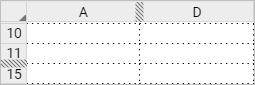
Hidden rows or columns are marked in the heading as shown:

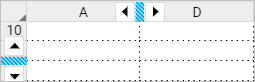
When you place the cursor over the marker indicating the hidden element, the heading will display two arrows indicating the direction in which the hidden element will be restored (before or after the marker).

To unhide a column or row, click on the desired arrow near the marker or select the two rows or columns between which the hidden element is located. To do this, click the first element and click the second element while holding the Shift key pressed. Unhide the element by executing the command in one of the ways:

1.In the Command menu, click Table > Unhide column or Unhide row.

2.Right-click the element heading and select Unhide from the context menu.

Freezing columns, rows and areas is used when working with large amounts of data. If you scroll the sheet to the right and/or down, the frozen row, column or area is always displayed on the screen. When you scroll through the sheet, the frozen element is separated from the other sheet elements with a bold line.

In MyOffice Spreadsheet, you can freeze the following elements:

•One or multiple columns: When you scroll the sheet to the right, only the frozen columns are displayed, and all columns that are to the left are hidden from the screen.

•One or multiple rows: When you scroll the sheet to the bottom, only the frozen columns are displayed, and all columns that are above are hidden from the screen.

•Columns and rows simultaneously: When you scroll the sheet to the right and down, only the frozen columns and rows are displayed, and all columns that are to the left and rows that are above are hidden from the screen.

•The area of the screen where the upper left cell is cell A1 and the lower right cell is the cell specified by the user.

To freeze the first row and/or the first column, choose one of the following ways:

•On the Table menu, select Freeze. In the opened sub-menu, select First row to freeze the top row, and/or First column to freeze the first column. If the window size does not allow to display the entire Toolbar, the command will be available by clicking the More button on the Toolbar.

•Click Freeze on the Toolbar. In the opened sub-menu, select Freeze first row to freeze the top row, and/or First first column to freeze the first column.

•Right-click the selected first column or first row header and select Freeze first row context menu command to freeze the top row and/or Freeze first column to freeze the first column.

To freeze one or more columns or one or more rows, follow these steps:

1.Select the desired columns/rows as a whole or select any number of cells located in those columns/rows.

2.Freeze rows or columns in one of the following ways:

•On the Table menu, select Freeze. In the opened sub-menu, select Freeze row <row number> to freeze rows, or Freeze column <column number> to freeze columns. If the window size does not allow to display the entire Toolbar, the command will be available by clicking the More button on the Toolbar.

•Click Freeze on the Toolbar. In the opened sub-menu, select Freeze row <row number> to freeze rows, or Freeze column <column number> to freeze columns.

•Right-click the selected column or row header and select the context menu command Freeze row <row number> to freeze the rows or Freeze column <column number> to freeze columns.

To freeze both rows and columns at the same time, follow these steps:

1.Select any number of cells located in the columns/rows you want to freeze.

2.Freeze rows or columns in one of the following ways:

•On the Table menu, select Freeze. In the opened sub-menu, select Freeze row <row number> and Freeze column <column number>.

•Click Freeze on the Toolbar. In the opened sub-menu, select Freeze row <row number> and Freeze column <column number>. If the window size does not allow to display the entire Toolbar, the command will be available by clicking the More button on the Toolbar.

To freeze an area, do the following:

1.Select the cell that will become the bottom right cell of the area.

2.Freeze rows or columns in one of the following ways:

•On the Table menu, select Freeze. In the opened sub-menu, select Up to cell <cell number>.

•Click Freeze on the Toolbar. In the opened sub-menu, select Freeze up to cell <cell number>. If the window size does not allow to display the entire Toolbar, the command will be available by clicking the More button on the Toolbar.

To remove freezing of all columns and rows in the document, select Unfreeze in the list which can be opened in one of the following ways:

•On the Table menu, select Freeze.

•Click Freeze on the Toolbar.

•Context menu called by right-clicking on the selected row or column header.

If the frozen area takes the entire visible area of the screen, a window will open in the lower right corner warning you that the frozen area is larger than the web browser window. To scroll through the sheet, you must enlarge the window, zoom out on the page, or unfreeze the rows and columns. In the warning window, click the button:

•Unfreeze all to unfix all frozen areas in the document.

•Fit to window to zoom out to the desired size (the entire frozen area, three rows below and three columns to the right of the frozen area).

If the frozen area is so large that even at its smallest scale it will not fit in the screen, the warning window displays only the Unfreeze button, while the Fit to window button is not displayed.

Limitations:

•If you scroll to the right and/or down, the notes are not displayed.

•When you edit a cell, it is enlarged only within the frozen area and does not affect the size of cells located outside the frozen area.