Sort and filter

To select a range for sorting and filtering, do the following:

1.Select a range of cells which contains all data to be sorted and filtered.

2.On the Toolbar, click . Or, in the Command menu, select Data and click Filter.

The active sorting and filtering range range on the sheet looks as follows:

•Headers of rows and columns are highlighted in green.

•A green frame appears around the range.

The upper line of the range marked as is not involved in the sorting and filtering.

MyOffice Spreadsheet can automatically detect the sorting and filtering range if the cells adjacent to the selected one contain data. Data in adjacent cells can be of any format.

To automatically detect the range:

1.Select an empty cell bordering the range.

2.On the Toolbar, click  Filter. Or, in the Command menu, select Data and click Filter.

Using filtering, you can hide or unhide the selected cells in the column. You can use different filters for different columns.

To filter data, do the following:

1.Click in the upper cell of the column to be filtered.

2.In the opened window, check the boxes with values to be displayed in the column.

3.Click OK to apply the filter or Cancel.

To quickly select or deselect all items in the range, use the Select all option.

To filter cells by fill color, follow these steps:

1.Click the button in the top cell of the column in which you want to filter the data.

2.In the window that opens, select the Filter > By color filtering method. Filtering by color is available if there are cells filled with color in the range.

3.In the palette of colors available for filtering, select the fill color.

4.Click OK.

To return to displaying all cells in the column, reopen the filter settings window and click the Clear filter button.

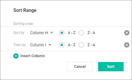
When sorting, the selected values in the column are arranged in the ascending (from A to Z) or descending (from Z to A) order. You can set different sorting criteria for each column.

To sort data in a column, do the following:

1.Click in the upper cell of the column.

2.In the opened setting window, select the sorting mode:

•Ascending: Sort the data in ascending order.

•Descending: Sort the data in descending order.

To sort data in a cell range, do the following:

1.Select a cell range which will contain all the data to be sorted. The range should consist of more than one line.

2.On the Toolbar, click  Sort. Or select Data of the Command menu and click Sorting order.

3.In the opened window, select the columns to which the sorting order will be applied and set the desired sorting mode for each of the columns (Sort Range).

4.By default, sorting is performed on the rightmost column. To add other columns, click Insert Column.

5.To sort according to the selected parameters, click Sort. To cancel the selection and close the Sort Range window, click Cancel.

To quickly select values to be used for filtering, use the Find box:

1.Select in the upper cell of the column that you want to filter.

2.In the opened window, enter the value that you want to find in the Find box.

3.Click in front of the values that you want to display in the column.

4.Click OK to apply the filter or Cancel to cancel the selection and close the window.

If the values in the selected range have changed, you can reapply a filter to the data without reconfiguring the filter itself. For this purpose:

1.On the Toolbar, click the  Filter. Or, in the Command menu, select Data.

2.Select the Reapply filter command from the drop-down menu.

To clear all the filters applied to the table, do the following:

1.Click  Filter on the Toolbar. Or, in the Command menu, select Data.

2.Select the Clear filter command from the drop-down menu.

To remove the current Sort and Filter range, on the Toolbar, click  Filter.